Neural networks are a fundamental technology driving many advancements in artificial intelligence (AI) and machine learning. Modeled after the structure and functionality of the human brain, neural networks excel at recognizing patterns, making decisions, and solving complex problems. Their applications span diverse fields, including healthcare, finance, entertainment, and beyond.
At its core, a neural network is a computational system inspired by the biological networks of neurons in the brain. It consists of layers of interconnected nodes (neurons), each designed to process and transmit information. Neural networks are typically categorized into three main layers:
- Input Layer: This layer receives the raw data input.
- Hidden Layers: These intermediate layers process the data using mathematical functions. The more layers and neurons, the more complex patterns the network can identify—a concept known as deep learning.
- Output Layer: This layer produces the final result, whether it’s a prediction, classification, or decision.
Neural networks operate by passing data through layers of neurons. Each connection between neurons has a weight, representing its importance. The steps involved include:
- Forward Propagation: Input data flows through the network, with each neuron applying an activation function to determine the output.
- Loss Calculation: The difference between the predicted output and the actual value (error) is measured using a loss function.
- Back Propagation: The network adjusts the weights of its connections by minimizing the error, using optimization techniques like gradient descent.
Neuron
The concept of a neuron is at the heart of artificial intelligence (AI), particularly in neural networks. Inspired by biological neurons in the human brain, an artificial neuron is a mathematical function that processes and transmits data. This seemingly simple unit is the fundamental building block of complex AI systems, enabling machines to learn, recognize patterns, and make decisions.
An artificial neuron, often called a “node” or “unit,” mimics the functionality of its biological counterpart. In the brain, neurons receive signals, process them, and transmit them to other neurons. Similarly, in AI, artificial neurons take numerical inputs, apply a transformation, and pass the result to other neurons in a network.
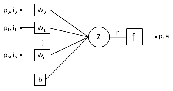
An artificial neuron has three main components:
Inputs
Represent features or data points.
Each input px , ix is associated with a weight wx , signifying its importance. The input px is connected to a neuron in previous layer and input ix is connected to the raw input data of the network depending on the layer.
Node
Aggregates the weighted inputs wx and adds a bias term b.
The aggregation z is often a summation:
z = \sum (w_x \: p_x) + b = n
Activation Functions
Applies a nonlinear transformation to the aggregated input.
Determines the neuron’s output, making the network capable of learning complex patterns.
The activation function introduces non-linearity, enabling the network to model complex relationships in data. Based on the activation function F the result will be buffered either in p or a.
Common activation functions include:
Sigmoid
Outputs values between 0 and 1. Ideal for binary classification.
f(z) = p = \frac{1}{1+exp\left(-z\:\frac{1}{T}\right)} The Sigmoid function f(z) is shown below with parameter T=1.
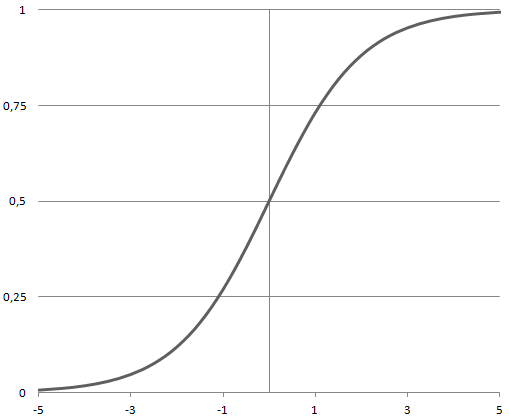
The function is differentiable and provides a smooth gradient, i.e., preventing jumps in output values. This is represented by an S-shape of the Sigmoid activation function. The derivative of the function is:
\frac{\partial p}{\partial z} = \frac{1}{T}\left(f(z) (1 - f(z)\right)The loss function commonly associated with the Sigmoid activation function is the binary entropy loss L, particularly for binary classification problems. Here’s how it is calculated:
L(y,p)=-\frac{1}{M}\sum_{m=0}^{M-1}\left(y_m\:log(p_m)+(1-y_m)\:log(1-p_m)\right)The formula calculates the loss for each individual net output sample p and then averages these losses over all samples.
ReLU (Rectified Linear Unit)
Outputs the input directly if positive; otherwise, outputs zero. Used extensively in deep networks due to its simplicity and efficiency.
f(z) = p = max(0,z)
The neurons in following layers will be deactivated if the output of the linear transformation is less than 0. Since only a certain number of neurons are activated, the ReLU function is far more computationally efficient when compared to the sigmoid and tanh functions.
ReLU accelerates the convergence of gradient descent towards the global minimum of the loss function due to its linear, non-saturating property.
All the negative input values become zero immediately, which decreases the model’s ability to fit or train from the data properly. Due to this reason, during the Backpropagation process, the weights and biases for some neurons are not updated. This can create dead neurons which never get activated. This is called as Dying ReLU problem.
Leaky ReLU
Leaky ReLU is an improved version of ReLU function to solve the Dying ReLU problem as it has a small positive slope in the negative area.
f(z) = p = max(az,z) \xrightarrow{a=0.01} max(0.01z,z)The advantages of Leaky ReLU are same as that of ReLU, in addition to the fact that it does enable Backpropagation, even for negative input values.
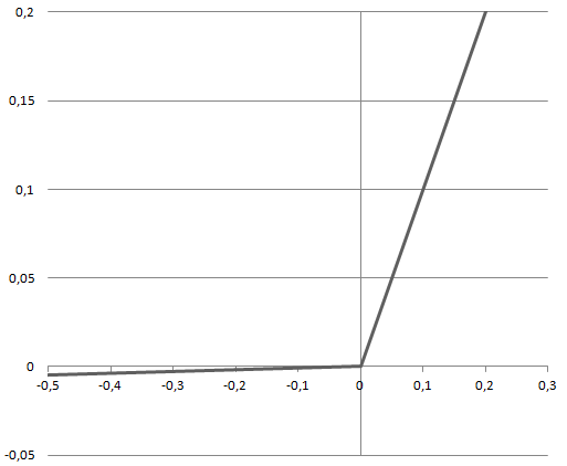
By making this minor modification for negative input values, the gradient of the left side of the graph comes out to be a non-zero value. Therefore dead neurons will be no longer encountered in that region.
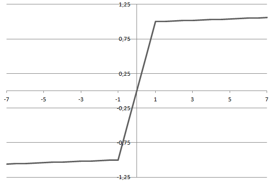
PLU (Piecewise Linear Unit)
The Piecewise Linear Unit (PLU) is a hybrid of tanh and ReLU and shown to outperform the ReLU on a variety of tasks while avoiding the vanishing gradients issue of the tanh.
f(z) = p = sgn(z) \cdot min(|z|, (a \: |z|) + b) \xrightarrow{a=0.01,\:b=1-a} sgn(z) \cdot min(|z|, (0.01 \: |z|) + 0.99)Piecewise linear functions handle the depth of modern neural networks well because they do not compress large values, preserving information and allowing the network to learn complex representations.
SoftMax
The SoftMax function converts a vector of raw scores (logits) into a probability distribution, where the probabilities of each class sum to 1. This makes the SoftMax function ideal for multi-class classification problems. SoftMax is typically used in the output layer of a neural network shown in block “s” below for multi-class classification. It assigns probabilities to each class (k=4 classes shown in below figure), and the class with the highest probability is often selected as the prediction.
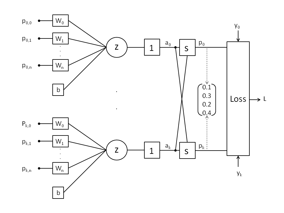
The SoftMax function is defined as:
f(s)=p_k=\frac{e^{a_k}}{\sum\limits_{m=0}^{M-1}e^{a_m}}The output of the SoftMax function for any input vector is a probability distribution. Each output lies between 0 and 1 and the sum of all outputs equals 1.
The loss function commonly associated with the SoftMax activation function is the categorical cross entropy loss L, particularly for multi-class classification problems. Here’s how it is calculated:
L(y,p)=\sum_{m=0}^{M-1}-y_m\:log(p_m)When combining SoftMax with the cross entropy loss, the derivative simplifies significantly. For a single data point, the gradient of the loss with respect to the SoftMax result p is:
\frac{\partial L}{\partial z}=-y_k+p_k\sum_{m=0}^{M-1}y_m=p_k-y_kBack Propagation
Back Propagation is a fundamental algorithm used to train neural networks by minimizing the error or loss between predicted and actual outputs. It calculates the gradient of the loss function with respect to the network’s weights and biases, enabling efficient weight updates via gradient descent or related optimization algorithms.
Output Layer Gradients
Calculate the delta of the loss with respect to the output layer’s activations. Multiply this delta value by the derivative of the output layer’s activation function to get the gradient:
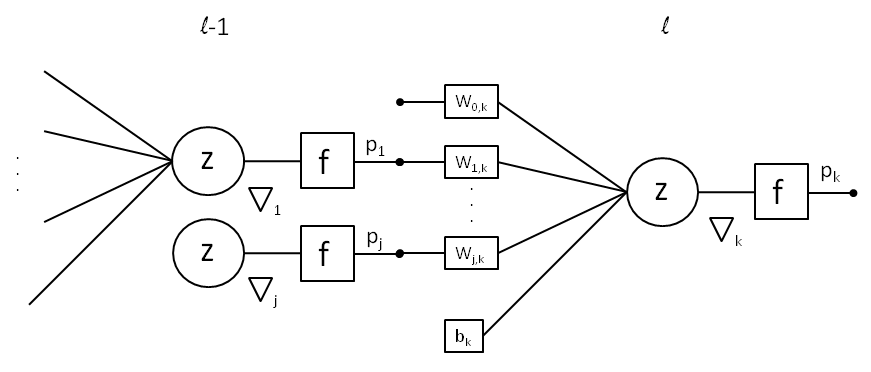
\nabla_k=(p-y)\:\frac{\partial p}{\partial z}\bigg|_kHidden Layer Gradients
For each hidden layer use the chain rule to propagate gradients where l is the layer index:
\nabla_j^{(l-1)}=\frac{\partial p^{(l-1)}}{\partial z}\bigg|_j\:\sum_kw_{j,k}^{(l)}\nabla_k^{(l)}Continue propagating gradients backward through all layers until reaching the input layer.
Weight and Bias Updates
Initialize weights and bias values by random values. The size of the weights values should be decreased by increasing number of net nodes.
Using the calculated gradients, update the weights w and biases b with an optimization algorithm such as Stochastic Gradient Descent (SGD):
w_{j,k}^{(l)}[n]=w_{j,k}^{(l)}[n-1]-\beta\:\nabla_k^{(l)}p_j^{(l-1)}b_{k}^{(l)}[n]=b_{k}^{(l)}[n-1]-\beta\:\nabla_k^{(l)}Where the learning rate β is defined by a value between 0 … 1.
Rules for Building Neural Network
- Scale the data so that min/max values of the inputs have been scaled to -1/1 or 0/1 based on the activation functions used
- Start with one or two hidden layers based on complexity. For less number of inputs (less complexity) start with one hidden layer.
- Number of the first hidden layer depends on the complexity of the input data. For high complexity increase the number of first hidden layer. The next layer size as half of the previous.
- Use ReLU, Leaky ReLU or PLU for intermediate layers.
- For output layer use Sigmoid for binary or multi-label classification, SoftMax for multi-class classifier, and Linear for regression.
- Split data for training and for testing the network.
- For binary classification (Sigmoid activation function) use binary cross entropy.
For multi-class, use categorical cross entropy. For regression (Linear activation function) use mean squared error.
Implementation
Neural network implementations involve building models from scratch in C# or Python for a foundational understanding, or using high-level deep learning frameworks like TensorFlow and PyTorch for more complex and efficient projects
Building from scratch using C#
The C# implementation demonstrates the principles of Neural Network modeling and training. With the help of a GUI the Neural Network can be modeled and the training can be observed. With the trained model the accuracy of the model can be shown using test data. Modeling and training using the GUI will be shown in the Example chapter below.
Followed C# code sections for the implementation of Net creation and Backpropagation algorithm using Gradient calculation and Weights update is shown.
The function “createNet” implements the Net topology the user can configure by the GUI. In the examples chapter two different configurations will be shown.
public void createNet(List<int> topology, List<ActFctType> actuatFct)
{
    tplgy = topology;
    actFct = actuatFct;

    symmetricRange = true;

    int numLayers = topology.Count;
    layers = new List<List<Neuron>>();
    List<double> weights = new List<double>();

    output = new List<double>();
    inputMax = new List<double>();
    inputMin = new List<double>();
    inputScaled = new List<double>();
    for (int i = 0; i < topology.ElementAt(0); i++)
    {
        inputMax.Add(-1000000.0);
        inputMin.Add(1000000.0);
    }

    for (int j = 0; j < (actFct.Count-1); j++)
    {
        if ((actFct.ElementAt(j) == Net.ActFctType.ReLu) ||
            (actFct.ElementAt(j) == Net.ActFctType.LeReLu))
        {
            symmetricRange = false;
        }
    }

    int numEntries = 0;
    for (int layerNum = 0; layerNum < numLayers; layerNum++)
    {
        List<Neuron> Neurons = new List<Neuron>();
        layers.Add(Neurons);

        for (int neuronNum = 0; neuronNum < topology.ElementAt(layerNum); neuronNum++)
        {
            Neuron neuron;

            double bias = 0.0;
            numEntries++;
            weights.Clear();

            if (layerNum == 0)
            {
                neuron = new Neuron(Net.ActFctType.Linear);

                weights.Add(1.0);
                numEntries++;
            }
            else
            {
                neuron = new Neuron(actFct.ElementAt(layerNum - 1));

                for (int i = 0; i < topology.ElementAt(layerNum - 1); i++)
                {
                    weights.Add(randomWeight());
                    numEntries++;
                }
            }
            neuron.initWeights(weights);
            if ((layerNum == (numLayers - 1)) &&
                (symmetricRange == false) &&
                (actFct.ElementAt(layerNum - 1) == Net.ActFctType.Sigmoid))
            {
                neuron.setParams(1.0, -2.0);
            }
            neuron.initBias(bias);
            layers.Last().Add(neuron);
        }
    }
}The function “backProp” implements the Backpropagation algorithm. The algorithm consists of calculating the gradients of the layers and updating the weights.
public void backProp(List<double> targetOut, double beta, double weightsLimit)
{
    // Calc Gradients of last Layer
    for (int n = 0; n < layers.Last().Count; n++)
    {
        layers.Last()[n].calcGradient(targetOut, n);
    }

    // Calc Gradients of hidden Layers
    for (int layerNum = layers.Count - 2; layerNum > 0; layerNum--)
    {
        List<Neuron> act = layers[layerNum];
        List<Neuron> right = layers[layerNum + 1];

        for (int n = 0; n < act.Count; n++)
        {
            act.ElementAt(n).calcGradient(right, n);
        }
    }

    // Update Weights for all layers
    for (int layerNum = layers.Count - 1; layerNum > 0; layerNum--)
    {
        List<Neuron> act = layers[layerNum];
        List<Neuron> left = layers[layerNum - 1];

        for (int n = 0; n < act.Count; n++)
        {
            act.ElementAt(n).updateWeights(left, beta, weightsLimit);
        }
    }

    return;
}The function “calcGradient” receives the Neuron layer as parameter and calculates the delta based on derived transfer function and the Neuron outputs sum of previous layer.
public void calcGradient(List<Neuron> layer, int act)
{
    double outputSum = 0.0;

    for (int n = 0; n < layer.Count; n++)
    {
        outputSum += (layer.ElementAt(n).weights[act] * layer.ElementAt(n).gradient);
    }

    double deltaGrad = outputSum * transferFctDeriv(net);
    gradient = deltaGrad;

    return;
}The weights and bias finally will be updated by function “updateWeights” using Stochastic Gradient Descent (SGD) method.
public void updateWeights(List<Neuron> layer, double beta, double weightsLimit)
{
    for (int n = 0; n < layer.Count; n++)
    {
        double weight = weights[n] - (beta * gradient * layer.ElementAt(n).prediction);
        if(Math.Abs(weight) < weightsLimit)
        {
            weights[n] = weight;
        }
    }
    bias = bias - (beta * gradient);

    return;
}The complete source code is available in Github.
Python using PyTorch Framework
PyTorch is a software-based open source deep learning framework used to build neural networks, combining the machine learning (ML) library of Torch with a Python-based high-level API.
A powerful Python Development Environment is Spyder. It provides advanced editing, interactive testing and debugging features. With Anaconda distribution the Python environment using packages among others PyTorch can be managed.
In principle a Neural Net using PyTorch can be modelled e.g. with 10 input nodes and 1 output node for prediction tasks as followed.
import torch

model = torch.nn.Sequential(
    torch.nn.Linear(10, 20),
    torch.nn.ReLU(),
    torch.nn.Linear(20, 5),
    torch.nn.ReLU(),
    torch.nn.Linear(5, 1),
    torch.nn.Sigmoid()
)This example Net has 2 hidden layers using ReLU activation function with 20 and 5 input nodes and one Sigmoid activation function for the prediction.
Following Python code shows training using MSE (Mean Squared Error) approach and Adam optimizer:
loss_fn = torch.nn.MSELoss()
optimizer = torch.optim.Adam(model.parameters(), lr=0.01)

for epoch in range(1000):
    for i in range(100):
        Xbatch = train_data.X[i:i+100]
        y_pred = model(Xbatch)
        ybatch = train_data.y[i:i+100]
        loss = loss_fn(y_pred, ybatch)
        optimizer.zero_grad()
        loss.backward()
optimizer.step()In this example a batch of data (train_data) will be trained for 100 iterations each epoch. The number of epochs and batch needs to be adjusted based on the training result.
Examples
Following examples are using datasets from Kaggle community to demonstrate prediction and classification tasks solved by neural networks.
Heart Disease Prediction
An example to demonstrate prediction task has been obtained by following dataset of the Kaggle community:
https://www.kaggle.com/datasets/rashikrahmanpritom/heart-attack-analysis-prediction-dataset
The task is to predict the chance of a heart attack based on different parameters shown below by:
| age | sex | chest pain type | resting blood pressure | cholesterol level | fasting blood sugar | resting ecg | max heart rate | exercise induced angina | ST depression | slope ST segment | number of major vessels | thalassemia types | target |
| 71 | 0 | 0 | 112 | 149 | 0 | 1 | 125 | 0 | 1.6 | 1 | 0 | 2 | 1 |
| 45 | 1 | 3 | 110 | 264 | 0 | 1 | 132 | 0 | 1.2 | 1 | 0 | 3 | 0 |
| 34 | 0 | 1 | 118 | 210 | 0 | 1 | 192 | 0 | 0.7 | 2 | 0 | 2 | 1 |
| 58 | 0 | 0 | 170 | 225 | 1 | 0 | 146 | 1 | 2.8 | 1 | 2 | 1 | 0 |
| : | : | : | : | : | : | : | : | : | : | : | : | : | : |
For the interpretation of the columns see the dataset description.
The manual coded Neural Network implementation in C# for this example uses following settings:
- Stochastic Gradient Descent based training
- MSE Loss function
- Simple Min/Max data normalization
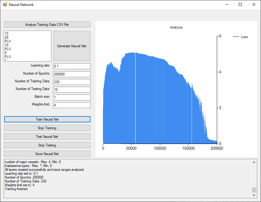
Based on the rules described in previous section the neural network for this task has been designed as followed:
13 Input nodes → 20 PLU → 10 PLU → 5 PLU → 1 Sigmoid
Note that different designs can have different impact on the quality of the result. Also the time needed to complete training successfully can vary.
With this neural network design a drop of the loss can be observed after about 180000 epochs using 230 data rows.
The performance of the trained network by 5 randomly chosen data rows will be shown below:
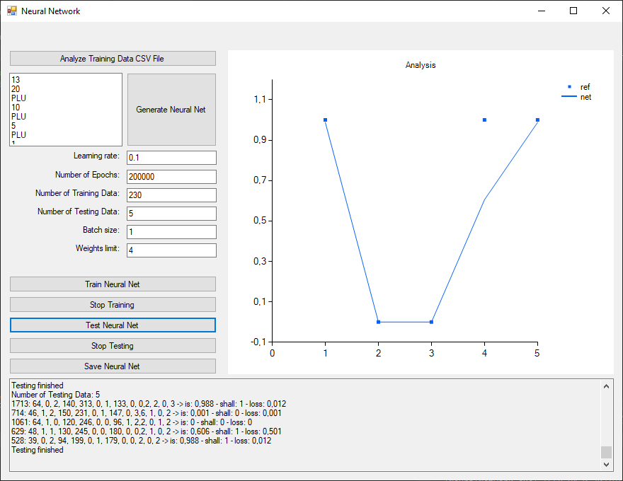
A deviation in 1 of the 5 data rows can be observed. Instead of a high chance (value 1) of heart attack the network rated it as 0.606 only.
| age | sex | chest pain type | resting blood pressure | cholesterol level | fasting blood sugar | resting ecg | max heart rate | exercise induced angina | ST depression | slope ST segment | number of major vessels | thalassemia types | target shall | target is |
| 64 | 0 | 2 | 140 | 313 | 0 | 1 | 133 | 0 | 0.2 | 2 | 0 | 3 | 1 | 0.988 |
| 46 | 1 | 2 | 150 | 231 | 0 | 1 | 147 | 0 | 3.6 | 1 | 0 | 2 | 0 | 0.001 |
| 64 | 1 | 0 | 120 | 246 | 0 | 0 | 96 | 1 | 2.2 | 0 | 1 | 2 | 0 | 0 |
| 48 | 1 | 1 | 130 | 245 | 0 | 0 | 180 | 0 | 0.2 | 1 | 0 | 2 | 1 | 0.606 |
| 39 | 0 | 2 | 94 | 199 | 1 | 1 | 179 | 0 | 0 | 2 | 0 | 2 | 1 | 0.988 |
The neural network simulator used for this example can be downloaded here.
Using PyTorch with a Neural Net model for prediction purposes
13 Input nodes → 25 ReLU → 10 ReLU → 1 Sigmoid
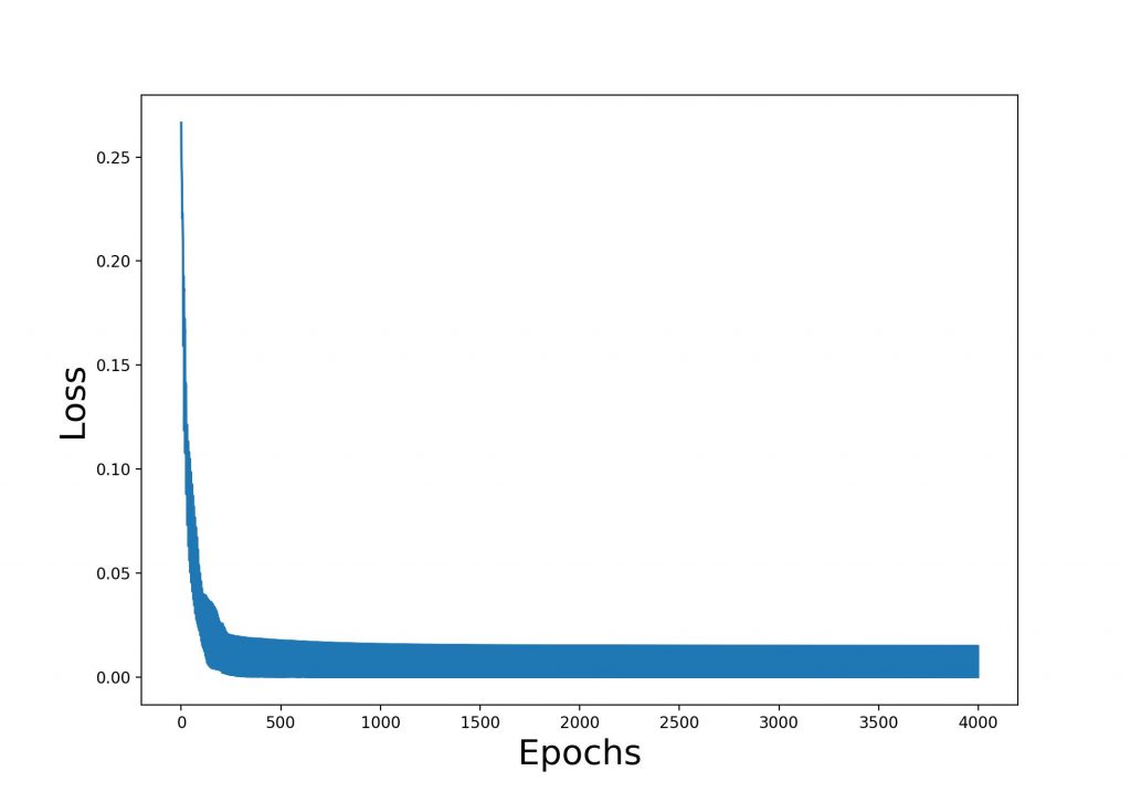
and a setup using Adam optimizer, Mean Squared Error Loss function and a data normalization done by Mean and Standard Deviation an accuracy of about 87% can be achieved. The Python script can be downloaded here. The Loss curve during the training is shown below.
Neural networks are highly effective for solving prediction tasks across a wide range of domains, thanks to their ability to model complex, non-linear relationships in data. Their effectiveness depends on the type of task, the quality of the data, and the architecture of the network.
Weather Type Classification
An example to demonstrate classification task has been obtained by following dataset of the Kaggle community:
https://www.kaggle.com/datasets/nikhil7280/weather-type-classification
The task is to predict the weather type based on different parameters shown below by:
| temperature | humidity | wind speed | precipitation (%) | cloud cover | atmospheric pressure | uv index | season | visibility (km) | location | weather type |
| 14 | 73 | 9.5 | 82 | partly cloudy | 1010.82 | 2 | winter | 3.5 | inland | rainy |
| 39 | 96 | 8.5 | 71 | partly cloudy | 1011.43 | 7 | spring | 10 | inland | cloudy |
| 30 | 64 | 7 | 16 | clear | 1018.72 | 5 | spring | 5.5 | mountain | sunny |
| -9 | 49 | 1.5 | 58 | partly cloudy | 1132.2 | 8 | spring | 16.5 | mountain | snowy |
| : | : | : | : | : | : | : | : | : | : | : |
For the interpretation of the columns see the dataset description.
Based on the rules described in previous section the neural network for this task has been designed as followed:
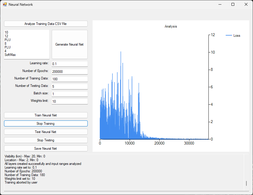
10 Input nodes → 12 PLU → 8 PLU → 4 SoftMax
Note that different designs can have different impact on the quality of the result. Also the time needed to complete training successfully can vary.
With this neural network design a drop of the loss can be observed after about 15000 epochs using 180 data rows.
The performance of the trained network by 5 randomly chosen data rows will be shown below:
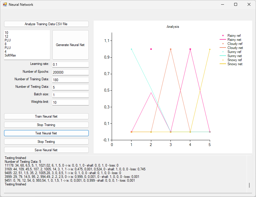
A deviation in 1 of the 5 data rows can be observed. Instead of 100% rainy the network rated it to 47.5% rainy only.
| temperature | humidity | wind speed | precipitation (%) | cloud cover | atmospheric pressure | uv index | season | visibility (km) | location | weather type shall | weather type is |
| 34 | 68 | 6.5 | 5 | 1 (clear) | 1021.02 | 6 | 1 (spring) | 5 | 0 (inland) | 100% sunny | 100% sunny |
| 44 | 109 | 45.5 | 107 | 2 (overcast) | 1005 | 14 | 3 (autumn) | 1 | 1 (mountain) | 100% rainy | 47.5% rainy 52.4% sunny 0.1% cloudy |
| 22 | 51 | 1.5 | 35 | 2 (overcast) | 1005.28 | 3 | 0 (winter) | 8.5 | 1 (mountain) | 100% cloudy | 100% cloudy |
| 29 | 79 | 14.5 | 95 | 2 (overcast) | 994.49 | 2 | 2 (summer) | 2.5 | 0 (inland) | 100% rainy | 99.9% rainy 0.1% sunny |
| 0 | 76 | 12 | 54 | 0 (partly cloudy) | 993.54 | 1 | 0 (winter) | 1.5 | 1 (mountain) | 100% snowy | 0.1% cloudy 99.9% snowy |
The neural network simulator used for this example can be downloaded here.
Using PyTorch with a Neural Net model for classification purposes
10 Input nodes → 12 ReLU → 8 ReLU → 4 Linear Output nodes
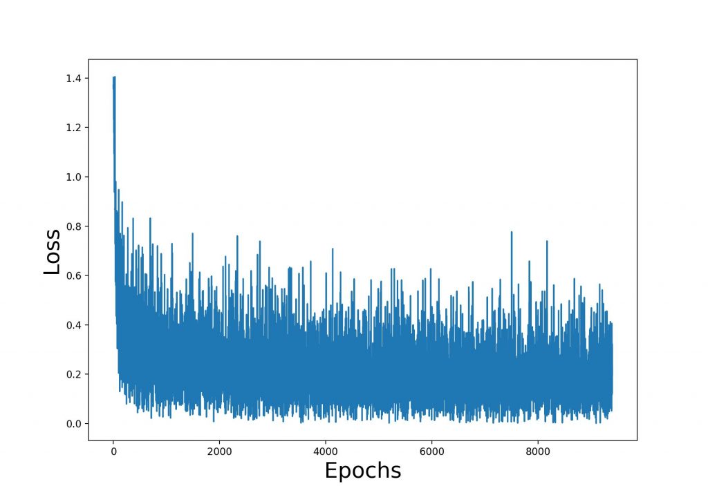
and a setup using Adam optimizer, Cross Entropy Error Loss function and a data normalization done by Mean and Standard Deviation an accuracy of about 92% can be achieved. The Python script can be downloaded here. The Loss curve during the training is shown below.
Neural networks are exceptionally well-suited for solving classification tasks across diverse domains, often delivering state-of-the-art performance. Their effectiveness stems from their ability to learn complex, non-linear patterns and extract hierarchical features directly from raw data. Here’s an assessment of their strengths, challenges, and performance for classification tasks.

Wonderful, what a website it is! This web site provides valuable facts to us,
keep it up.
Really appreciate it!