Mean filtering is an important method for noise reduction in analog signals. It is commonly used in signal processing to remove signal distortions that may result from noise or interference.
The basic principle of mean filtering is signal smoothing through the use of an average. The method involves taking a certain number of consecutive signal values and averaging them to produce a single output that reflects the signal without the noise.
There are various types of mean filters.
Mean filtering is used in a variety of applications, from audio processing to industrial automation. Although it is relatively simple and fast, it is important to note that it also has some disadvantages. Mean filtering can result in the loss of important signal details and may cause a delay in the output signal. Therefore, when applying mean filters, the impact on the signal should be carefully considered.
In conclusion, mean filtering is an effective method for reducing noise in analog signals. It is a simple and fast method that can be applied in a wide range of applications. However, it is important to consider the impact of the filter on the signal, as it may lead to the loss of important signal details and a delay in the output signal.
Moving Average
The moving average method involves taking a sliding window of a specified size and moving it along the time series, with the window always containing the same number of data points. The average of the data points within the window is then calculated and used as the smoothed value for the data point. The process is repeated for all data points in the time series, resulting in a smoothed time series that eliminates short-term fluctuations and highlights long-term trends.
The moving average method can be used to remove noise and other irregularities in the data, making it easier to identify trends and patterns.
The size of the window used in the moving average calculation determines the degree of smoothing that is applied to the data. A smaller window will result in a more responsive, but more noisy, smoothed time series, while a larger window will result in a smoother, but less responsive, smoothed time series.
The moving average method involves calculating the average of a fixed number of consecutive data points, with each data point weighted equally.
y_{k}=\frac{1}{N}\sum_{n=0}^{N-1}x_{k-n} \\[5pt]
y_{k}=\frac{1}{N}x_k+y_{k-1}-\frac{1}{N}x_{k-N} \\[5pt]
y_{k}=y_{k-1}+\frac{1}{N}\left(x_{k}-x_{k-N}\right)
Equations left show the derivation from mean value calculation to moving average calculation. Note that the init sequence of moving average is important for the first N-values. Here the startup average values needs to be calculated based on the first N-values. If not done there will be resulting an offset which effects following iterations.
To improve this a simplification can be introduced showed above. This has the advantage that the average value calculation for the first N-values is not needed and there for an offset will not happen any more. The resulting equation is related to PT1-filter described in next chapter.
y_{k}=\frac{1}{N}\sum_{n=0}^{N-1}x_{k-n}\\[5pt]
y_{k}=\frac{1}{N}x_k+y_{k-1}-\frac{1}{N}x_{k-N}\\[5pt]
y_{k}=\frac{1}{N}x_k+y_{k-1}\frac{N-1}{N}\\[5pt]
y_{k}=y_{k-1}+\frac{1}{N}\left(x_{k}-y_{k-1}\right)
PT1 Filter
The PT1 Filter is a commonly used type of filter in signal processing for processing and analyzing digital signals. It is a simple and effective filter that is often used for smoothing and noise reduction of signals. It works by attenuating high-frequency components while allowing low-frequency components to pass through. The filter response is characterized by its time constant, which determines the rate at which the filter responds to changes in the input signal.
The PT1 Filter is particularly useful in digital signal processing applications where a signal is subject to noise or other unwanted high-frequency components. By reducing these unwanted components, the PT1 Filter can improve the accuracy and reliability of signal processing algorithms.
One of the advantages of the PT1 Filter is its simplicity and ease of implementation.
It requires only a small amount of memory and processing power, making it a cost-effective solution for many signal processing applications. Additionally, the PT1 Filter is a linear filter, which means that it preserves the shape of the input signal and does not introduce any distortion or nonlinear effects.
The PT1 Filter is commonly used as digital audio processing, image processing, and sensor signal conditioning.
In conclusion, the PT1 Filter is a widely used type of filter for processing and analyzing digital signals. It is a simple and effective filter that can improve the accuracy and reliability of signal processing algorithms by reducing unwanted high-frequency components. Its simplicity and ease of implementation make it a cost-effective solution for many signal processing applications.
Beginning with the Laplace equation for the PT1 Filter then applying the Laplace Transformation and with some mathematical transformations the PT1 Filter difference equation will be obtained.
Below the step response of the PT1 Filter is shown with K=1 and T=4ms
Y_{(s)} =  \frac{K}{1+T s} \: X_{(s)} \\[5pt]
Y_{(s)}+ T \: s\: Y_{(s)} = K \:X_{(s)} \:\: \origof \:\: y_{(t)}+T\:\dot{y}_{(t)}=K\: x_{(t)}\\[5pt]
y_{k}+T\:\frac{y_k-y_{k-1}}{dt}=K\: x_k\\[5pt]
y_{k}+\frac{dt}{T}\:y_k=y_{k-1}+K\:\frac{dt}{T}\:x_k\\[5pt]
y_{k}=\frac{T}{T+dt}\:y_{k-1}+K\:\frac{dt}{T+dt}\:x_k\\[5pt]
\frac{T}{T+dt}\:y_{k-1}=y_{k-1}-\frac{dt}{T+dt}\:y_{k-1}\\[5pt]
y_{k}=y_{k-1}+\frac{dt}{T+dt}\:\left(K\:x_k-y_{k-1}\right)\\[5pt]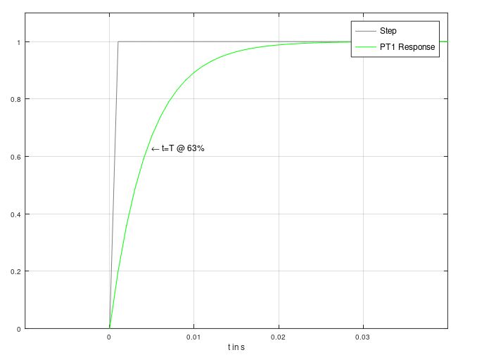
y_{k}=y_{k-1}+\frac{dt}{T+dt}\:\left(K\:x_k-y_{k-1}\right)\\[5pt]
K=1\\[5pt]
\frac{dt}{T+dt} = \frac{1}{N}\\[5pt]
y_{k}=y_{k-1}+\frac{1}{N}\left(x_{k}-y_{k-1}\right)\\[5pt]
PT1 Filter difference equation can be easily transformed to Moving Average filter by setting K-factor to 1 and replacing the ratio of sampling time dt/(T+dt) by number of sampling values 1/N.
Low Pass Filter
The A low pass filter is a fundamental type of filter used in signal processing to remove high-frequency components from a signal while preserving its low-frequency components. In signal processing, a low pass filter is often used to smooth out noise or to extract useful information from a signal.
The principle of a low pass filter is simple. It allows signals with frequencies below a certain cutoff frequency to pass through, while attenuating signals with frequencies above the cutoff frequency. The cutoff frequency is determined by the filter design and is typically expressed as a fraction of the signal’s sampling rate.
One of the most common types of low pass filters used in signal processing is the finite impulse response (FIR) filter. The FIR filter is a digital filter with a finite number of coefficients. It operates by convolving the input signal with the filter coefficients to generate the output signal. The cutoff frequency of an FIR filter is determined by the length and coefficients of the filter.
Another commonly used low pass filter in signal processing is the infinite impulse response (IIR) filter. The IIR filter is a recursive filter that uses feedback to generate the output signal. It is often used when a more aggressive attenuation of high-frequency components is required.
Low pass filters are particularly useful in signal processing applications where a signal is subject to noise or other unwanted high-frequency components. By reducing these unwanted components, low pass filters can improve the accuracy and reliability of signal processing algorithms.
One of the limitations of low pass filters in signal processing is that they can introduce phase distortion, especially at higher frequencies. This means that the filtered signal may be shifted in time relative to the original signal, which can be a problem for certain applications. Additionally, low pass filters can introduce ringing, which is a transient response that occurs when the filter is switched on or off.
In conclusion, low pass filters are an essential tool in signal processing for removing unwanted high-frequency components from signals. They are particularly useful in applications where a signal is subject to noise or other unwanted high-frequency components. The FIR filter and IIR filter are the two most commonly used low pass filters in signal processing, each with its own advantages and limitations. While low pass filters can introduce phase distortion and ringing, they are a necessary component of signal processing algorithms that improve the accuracy and reliability of the signal.
A First Order Low Pass Filter can be converted into a PT1 Filter with the K as gain factor and Time constant T.
After Z-Transformation and some conversions a Z-Transfer Function will be obtained.
The Z-Transfer Function can be transformed into a discrete time function with back Transformation.
The coefficient can now be calculated very easily.
The frequency response as an example is shown below.
H_{(s)} = \frac{2\pi f_c}{2\pi f_c+s}=\frac{1}{1+\frac{1}{2\pi f_c}s}= \frac{K}{1+T\:s}\\[5pt]
H_{(z)}=Z\big\{H_{(s)}  H_{0(s)} \big\} \\[5pt]
H_{(z)}=Z\bigg\{H_{(s)}  \frac{1}{s (1-e^{-s\:T_a})}\bigg\}=\frac{z-1}{z} Z\bigg\{\frac{H_{(s)}}{s}\bigg\}\\[5pt]
Z\bigg\{\frac{1}{s}\bigg\}=\frac{z}{z-1}
Z\bigg\{\frac{a}{a+s}\bigg\}=\frac{1-e^{-a\:T_a}}{z-e^{-a\: T_a}}\\[5pt]
H_{(z)}=\frac{z-1}{z} \frac{z}{z-1} K \frac{1-e^{-\frac{T_a}{T}}}{z-e^{-\frac{T_a}{T}}}=K \frac{1-e^{-\frac{T_a}{T}}}{z-e^{-\frac{T_a}{T}}}\\[5pt]
H_{(z)}=\frac{K(1-e^{-\frac{T_a}{T}}) z^{-1}}{(z-e^{-\frac{T_a}{T}}) z^{-1}}\\[5pt]
H_{(z)}=\frac{b_0+b_1\:z^{-1}}{a_0+a_1\:z^{-1}} \:\: \origof \:\: y_k=b_1\:u_{k-1}-a_1\:y_{k-1}\\[5pt]
y_k\approx b_1\:u_{k}-a_1\:y_{k-1}\\[5pt]
b_0=0, b_1=K(1-e^{-\frac{T_a}{T}}),\\[5pt]
a_0=1 (\rightarrow normed), a_1=-e^{-\frac{T_a}{T}}\\[5pt]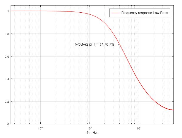
Median Filter
A median filter is a commonly used type of signal processing filter that is used to remove noise from a signal. It works by replacing each data point in a signal with the median value of its neighboring data points, thus smoothing out any spikes or fluctuations in the signal.
In signal processing, median filters are used to remove random noise from signals without distorting the underlying signal too much. They are particularly useful in situations where the noise is not Gaussian, as other types of filters such as low-pass filters may not be effective in removing non-Gaussian noise.
The principle of a median filter is simple. For each data point in a signal, a window of neighboring data points is selected. The median value of the data points within the window is then calculated and assigned to the original data point. The size of the window determines the level of smoothing that the filter applies to the signal. Larger windows result in greater smoothing, but may also lead to a loss of detail in the signal.
One of the advantages of median filters is their ability to preserve sharp features in a signal, such as edges and corners. This is because the median value of a set of data points is not affected by outliers, whereas other types of filters such as mean filters can be skewed by outliers.
Median filters are widely used in image processing applications, where they are used to remove noise from images while preserving the sharpness of edges and other features. They are also used in audio signal processing, where they are used to remove noise from recordings.
One of the limitations of median filters is that they can introduce ringing artifacts in the filtered signal. This occurs when the window size is too large and the filter smooths out sharp features in the signal. Additionally, median filters can be computationally expensive, especially for large data sets.
In conclusion, median filters are a valuable tool in signal processing for removing noise from signals while preserving the underlying structure of the signal. They are particularly useful in situations where the noise is non-Gaussian or when sharp features in the signal need to be preserved. However, their use can also lead to ringing artifacts and they can be computationally expensive. Despite these limitations, median filters remain a valuable and widely used tool in signal processing applications.
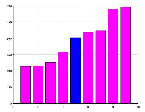
In the example shown on the right side the Median Filter takes for every sample point the last 9 sampled values. After sorting, the value in the middle will be taken as output of the Filter.
Morphological Operators
Morphological operators are mathematical operations that are commonly used in signal processing to manipulate and analyze images and signals. The two most commonly used morphological operators are erosion and dilation.
Erosion is a morphological operation that is used to shrink the boundaries of an image or signal. In signal processing, erosion is often used to remove small features or to separate two adjacent objects that are too close together. The operation involves sliding a small, predefined kernel or structuring element over the image or signal, and removing all pixels or data points that do not meet a specific criterion.
For example, in a binary image, if the criterion is set to “all pixels in the structuring element must be set to 1”, erosion will remove any pixels in the image that are not surrounded by other pixels that are also set to 1. This can be useful for removing small objects or for separating two objects that are too close together.
Dilation, on the other hand, is a morphological operation that is used to expand the boundaries of an image or signal. In signal processing, dilation is often used to fill small holes or gaps in an image or to merge adjacent objects that are too close together.
The operation involves sliding a small kernel or structuring element over the image or signal, and setting all pixels or data points that meet a specific criterion to a particular value.
For example, in a binary image, if the criterion is set to “at least one pixel in the structuring element must be set to 1”, dilation will set all pixels in the image that are adjacent to pixels that are set to 1 to 1 as well. This can be useful for filling small holes or gaps in an image or for merging adjacent objects that are too close together.
Erosion and dilation can be used in combination with each other to perform more complex operations, such as opening and closing. Opening involves performing an erosion followed by a dilation, and is often used to remove small objects or to smooth out the edges of larger objects. Closing involves performing a dilation followed by an erosion, and is often used to fill small gaps or to connect nearby objects.
In conclusion, erosion and dilation are two commonly used morphological operators in signal processing that are used to manipulate and analyze images and signals.
Erosion is used to shrink the boundaries of signal, while dilation is used to expand the boundaries.
These operations will be used in combination with a mean value calculation.
With the structure component B the Dilation and Erosion operations can be adapted properly.
Below a filtered signal by Erosion and Dilation is shown with the values for structue components on the right side.
Dilation: \\(X\oplus B_1)[n] = \max_{\substack{m=0,..M-1}}\Bigg\{X[n+m-M]-B_1[m]\Bigg\} \\[5pt]
Erosion: \\ (X\ominus B_2)[n] = \min_{\substack{m=0,..M-1}}\Bigg\{X[n+m-M]-B_2[m]\Bigg\} \\[5pt]
\\[15pt]
X=\frac{1}{2}\big [(X\oplus B_1) \, + (X\ominus B_2) ] \\[5pt]
B_1=[10, 5, 0, 5, 10] \\[5pt]
B_2=[\text{-}10, \text{-}5, 0, \text{-}5, \text{-}10]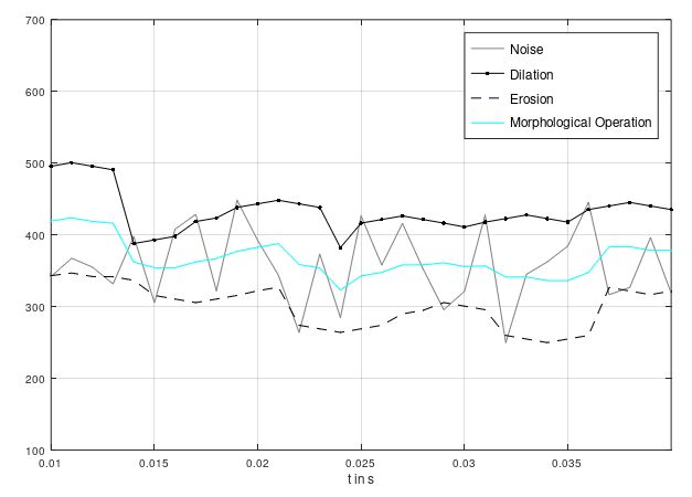
Summary
Every Filter type shown above can be used for Mean Filtering. The decision which Filter shall be used depends on run time consumption and the requirements on the filtered signal.
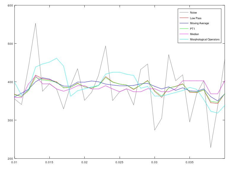
The Examples above were implemented in Octave and will be shown below. The corresponding m-file can also be downloaded here.
% The sampling frequency in Hz.
Fs = 1000;
% Sampling time
T = 1/Fs;
% Buffer length
L = 300;
% Create a time base
t = (0:L-1)*T;
input = 400*sin(2*pi*5*t+pi/3) + 60*randn(size(t));
% moving average
moving_average = input;
N = 10;
moving_average(N) = (1/N)*(sum(input(1:N)));
for i=N+1:L
  moving_average(i) = moving_average(i-1) + ((1/N)*(input(i) - input(i-N)));
end
% pt1 filter
pt1_filter = input;
K = 1;
Tau = (5*T)-T;
for i=2:L
  pt1_filter(i) = pt1_filter(i-1) + ((T/(Tau+T))*(K*input(i) - pt1_filter(i-1)));
end
input_response = zeros(1,L);
pt1_filter_response = input_response;
for i=2:L
  input_response(i) = 1;
  pt1_filter_response(i) = pt1_filter_response(i-1) + ((T/(Tau+T))*(K*input_response(i) - pt1_filter_response(i-1)));
end
% LP first order
lp_filter = input;
b = K*(1-exp(-(T/Tau)));
a = -exp(-(T/Tau));
for i=2:L
   lp_filter(i) = b*input(i) - a*lp_filter(i-1);
end
% Median filter
median_filter = input;
median_sorted = zeros(1,9);
M = 9;
for i=M:L
   med_vals = input(i-M+1:i);
   med_vals_sort = sort(med_vals);
   if( i == 50 )
    median_sorted = med_vals_sort;
   endif
   median_filter(i) = med_vals_sort(((M/2)+0.5));
end
% Morphological filter
morph_filter = input;
FilterMax = input;
FilterMin = input;
Mask1 = [10 5 0 5 10];
Mask2 = [-10 -5 0 -5 -10];
for i=5:L
  masked = input(i-4:i)-Mask1(1:5);
  FilterMax(i) = max(masked);
  masked = input(i-4:i)-Mask2(1:5);
  FilterMin(i) = min(masked);
  morph_filter(i) = (FilterMax(i)+FilterMin(i))/2;
end