Regression analysis is a fundamental statistical method used to understand the relationship between one dependent variable and one or more independent variables. It’s a powerful tool in data analysis and predictive modeling, widely used across various fields such as economics, finance, psychology, and more. In this article, we’ll delve into the world of regression models, exploring their types, applications, and key concepts.
Regression analysis aims to model the relationship between a dependent variable (Y) and one or more independent variables (X). The primary goal is to predict the value of the dependent variable based on the values of the independent variables. It helps in understanding how changes in the independent variables are associated with changes in the dependent variable.
Types of Regression Models (bold marked Models discussed in this blog):
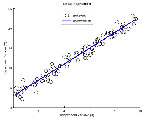
- Simple Linear Regression: This is the simplest form of regression involving a single independent variable. The relationship between the independent and dependent variables is assumed to be linear.
- Multiple Linear Regression: In this model, there are multiple independent variables, but the relationship with the dependent variable is still linear.
- Polynomial Regression: When the relationship between the variables is not linear, polynomial regression fits a polynomial equation to the data.
- Logistic Regression: Unlike linear regression, logistic regression is used when the dependent variable is categorical. It predicts the probability of occurrence of an event by fitting data to a logistic curve.
- Ridge Regression and Lasso Regression: These are techniques used to handle multicollinearity and prevent overfitting by adding regularization terms to the regression equation.
- Time Series Regression: This model is used when the data involves time-dependent variables. It helps in forecasting future values based on historical data.
Applications of Regression Models:
- Predictive Modeling: Regression analysis is widely used in predictive analytics to forecast future trends and outcomes based on historical data.
- Risk Management: In finance and insurance, regression models are used to assess and manage risks by predicting the likelihood of certain events.
- Marketing Analytics: Regression analysis helps marketers understand the relationship between marketing efforts and outcomes such as sales, customer acquisition, and retention.
- Healthcare: Regression models are employed in medical research to analyze the factors influencing health outcomes and predict patient outcomes.
- Economics: Econometric models use regression analysis to study the relationships between economic variables such as GDP, inflation, and unemployment.
Multiple Linear Regression
Multiple linear regression is an extension of simple linear regression that allows us to model the relationship between a single dependent variable and multiple independent variables. This technique is used to understand how the dependent variable changes as each of the independent variables changes, while controlling for the influence of the other independent variables in the model.
The general form and the matrix representation of the multiple linear regression model with an example of one variable x (k=2) is shown below
\hat{y} = \theta_0 + \theta_1 \: x \:\: \rightarrow \:\: \hat{Y} = \Theta^T \: X\\[10pt]
\hat{Y}_{1,n} =\Theta^T_{1,k} \: X_{k,n} \:\: \xrightarrow{k=2} \:\: \hat{Y}_{1,n} =\begin{bmatrix}
\theta_0 & \theta_1 \\
\end{bmatrix} \: \begin{bmatrix}
1 & 1 & \dots & 1 \\
x^{(1)} & x^{(2)} & \dots & x^{(n)} \\
\end{bmatrix}\\[5pt]
Multiple linear regression relies on several key assumptions. The relationship between the dependent variable and each independent variable is linear. Observations are independent of each other. The prediction error expectation value is zero (freedom of systematic faults in prediction error):
E(Y) = E(\hat{Y}) + E(\bold{e})\\[5pt]
\bold{e} \sim \mathcal{N}(0,\sigma^{2})\\[5pt]
E(Y) = E(\Theta^T \: X) + E(\mathcal{N}(0,\sigma^{2}))=E(\Theta^T \: X)\\[5pt]
The variance of prediction error and dependent variable is constant:
Var(\hat{Y}) \sim \mathcal{N}(\Theta^T \: X,0)\\[5pt]
Var(Y) = Var(\hat{Y})+Var(\bold{e}) \\[5pt]
Var(Y) = Var(\mathcal{N}(\Theta^T \: X,0))+Var(\mathcal{N}(0,\sigma^{2}) =\sigma^{2}=Var(\bold{e})\\[5pt]
The error terms are normally distributed. Using a normal distribution for variable predictions with mean value µ and variance Sigma we obtain:
\mathcal{N}(\mu,\sigma)\:\rightarrow \;p(x|\mu,\sigma)=\frac{1}{\sigma\sqrt{2\pi}}\;exp\left(-\frac{1}{2}\left(\frac{x-\mu}{\sigma}\right)^2\right)Maximum Likelihood Estimation
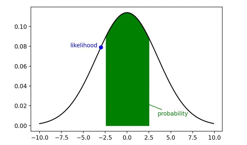
Before going into detail of this kind of estimation lets clarify what is the difference between Likelihood and Probability. See following normal distribution where Likelihood represents the plausibility of Mean value µ and Variance σ if value x occurs. Written as L(µ,σ|x). Hence it represents a y-value on the distribution curve.
Probability is an area below the curve. It describes how probable is the value x given the Mean value µ and Variance σ. Written as p(x|µ,σ). The Likelihood L(x) get its maximum at the mean value here L(x=µ=0)=0.11 where the Probability p(x) gets its maximum in a range of x-values here p(x>±10)=1.
The likelihood function measures how likely it is to observe the given data under various parameter values of the chosen statistical model. In other words it can be expressed by how probable is the evidence E if a Hypothesis occurs p(E|H). The Evidence here would be the to be predicted dependent variable y and the Hypothesis are the independent variable x and the model or distribution parameter µ, σ collected as θ. For the distribution the normal distribution is selected.
L(\mu,\sigma|x)=p(E|H)=p(y|x,\theta)=\mathcal{N}(E(x,\theta),\sigma)Since expectation value of dependent variable y will be predicted by the model the Mean value results in
E(Y) \approx E(\hat{Y})=E(\Theta^TX) = \Theta^TX
Maximum Likelihood Estimation (MLE) is a statistical method used for estimating the parameters of a probability distribution by maximizing a likelihood function. MLE seeks to find the parameter values that make the observed data most probable.
L(\Theta)=p(Y|X,\Theta) =p(y_1|x_1,\Theta)\:(y_2|x_2,\Theta)\dots p(y_M|x_M,\Theta)=\prod_{m=1}^{M}p(y_m|x_m,\Theta)The target of MLE is to find the parameter values that maximizes the likelihood function:
\hat{\Theta}_{MLE}=\underset{\Theta}{\mathrm{argmax}}\:L(\Theta)Putting things from above together the Likelihood for one dependent variable y and multi independent variable x can be calculated as followed:
\mathcal{N}(\Theta^TX,\sigma)\:\rightarrow \;p(y|x,\Theta^TX,\sigma)=\frac{1}{\sigma\sqrt{2\pi}}\;exp\left(-\frac{1}{2}\left(\frac{y-\Theta^TX}{\sigma}\right)^2\right)In practice, it is often easier to work with the logarithm of the likelihood function, known as the log-likelihood. This is because the log transformation turns the product of probabilities into a sum, simplifying the calculations:
ln\left(p(y|x,\Theta^T \: X,\sigma)\right)=-\frac{1}{2}ln\left(2\pi\right)-ln\left(\sigma\right)-\frac{1}{2\sigma^2}\left(y-\Theta^T \: X\right)^2\\[5pt]For multiple dependent variables Y and due to the fact that using logarithm of the Likelihood function multiplication become to addition it can be simplified as followed:
ln\left(p(Y|X,\Theta)\right)=-\frac{1}{2\sigma^2}\sum_{n=1}^{N}\left(y^{(n)}-h_\Theta(x^{(n)})\right)^2-\frac{N}{2}ln\left(2\pi\right)-N\:ln\left(\sigma\right)\\[5pt]Multiplying the log-likelihood with the variance and dividing it with the number of variables the first term of the result defines the cost function J. The log terms contributes to an offset only and thus can be ignored.
ln\left(L(\Theta)\right)\frac{\sigma^2}{N}=-\frac{1}{2N}\sum_{n=1}^{N}\left(y^{(n)}-h_\Theta(x^{(n)})\right)^2-ln\left(2\pi\sigma\right)-ln\left(\sigma^2\right)\\[5pt]
J(\Theta)=\frac{1}{2N}\sum_{n=1}^{N}\left(h_\Theta(x^{(n)})-y^{(n)}\right)^2\\[5pt]
To obtain the maximum log-likelihood the cost function needs to be derived. A representative matrix notation is shown below. Ideally the result will be zero at its maximum.
\frac{\partial J(\Theta)}{\partial\Theta}=-\frac{1}{N}\sum_{n=1}^{N}\left(y^{(n)}-h_\Theta(x^{(n)})\right)x^{(n)}=\frac{1}{N}\sum_{n=1}^{N}\left(h_\Theta(x^{(n)})-y^{(n)}\right)x^{(n)}\\[5pt]
\frac{\partial J(\Theta)}{\partial\Theta}=X^TX\:\Theta-X^TY\stackrel{!}{=}0
Gradient Descent Algorithm
The gradient descent algorithm is an optimization technique used to find to maximize the log-likelihood by iteratively adjusting the parameters of the model. It is widely used in machine learning and statistical modeling to find the optimal parameters that minimize the error between the predicted and actual values.
\Theta_k=\Theta_{k-1}-\beta\:\frac{\partial J(\Theta)}{\partial\Theta_{k-1}}\\[5pt]
\Theta_k=\Theta_{k-1}-\beta\:\left(X^TX\Theta_{k-1}-X^TY\right)
Bayesian Regression
Bayesian regression is a statistical technique that applies Bayesian principles to linear regression. In Bayesian inference, we update our beliefs about the parameters of a model based on observed data. This involves combining prior beliefs (prior distribution) or so called Hypothesis H with the Likelihood p(E|H) of the observed data or Evidence E to produce a posterior distribution p(H|E).
p(H|E) = \frac{p(E|H)\cdot p(H)}{p(E)}=\frac{likelihood\cdot p(prior)}{p(observation)}=p(posterior)Prior Distribution represents our beliefs about the parameters before observing any data. It is chosen based on prior knowledge or assumptions.
Likelihood Function represents the probability of the observed data given the parameters. In regression, this is typically based on a Gaussian (normal) distribution if we assume the residuals (errors) are normally distributed.
Posterior Distribution combines the prior distribution and the likelihood function, providing an updated belief about the parameters after observing the data. It is obtained using Bayes’ theorem
p(\Theta|Y) = \frac{p(Y|X,\Theta)\:p(\Theta)}{p(Y)} \sim p(Y|X,\Theta)\:p(\Theta)Target is to find similar to MLE the parameter values that maximizes the a-posteriori (MAP) probability by the likelihood function with prior beliefs (prior distribution).
\hat{\Theta}_{MAP}=\underset{\Theta}{\mathrm{argmax}}\:L(\Theta)\;p(\Theta)Lets assume that the prior distribution is based on a Gaussian (normal) distribution where the mean value is zero. The prior log-distribution is proportional to the squared parameters.
p(\Theta)=\mathcal{N}(0,\sigma^{2})=\frac{1}{\sigma\sqrt{2\pi}}\:exp\left(\frac{1}{2}\left(\frac{\Theta}{\sigma}\right)^2\right)\\[5pt]
ln(p(\Theta)=-\frac{1}{2}ln\left(2\pi\right)-ln\left(\sigma\right)+\frac{1}{2\sigma^2}\Theta^2\\[5pt]
ln(p(\Theta)\sim\frac{1}{2\sigma^2}\Theta^2
The log based cost function gets an additional term based on the posterior distribution calculation:
J(\Theta)=\frac{1}{2N}\sum_{n=1}^{N}\left(h_\Theta(x^{(n)})-y^{(n)}\right)^2+\frac{1}{2\sigma^2}\sum_{m=1}^{M}\Theta^2_mThe additional term is also known as a regularization term and will be introduced here with a const parameter λ:
J(\Theta)=\frac{1}{2N}\sum_{n=1}^{N}\left(h_\Theta(x^{(n)})-y^{(n)}\right)^2+\lambda\sum_{m=1}^{M}\Theta^2_mThe gradient descent algorithm is also extended by the regularization term as shown below.
\frac{\partial J(\Theta)}{\partial\Theta}=X^TX\:\Theta-X^TY+\lambda\:\Theta^T\ThetaExample
To demonstrate the Multiple Linear Regression the dataset Housing Price Prediction from https://www.kaggle.com/ homepage will be used.
An extraction of the data content some rows are shown in the table below.
| Price in Euro | Area in qm | Bedrooms | Bathrooms | Stories | Main Road | Guestrooms | Basement | Gas Heating | Air Conditioning | Parking | Preferred Area | Furnishing |
|---|---|---|---|---|---|---|---|---|---|---|---|---|
| 134750 | 832 | 4 | 4 | 4 | 1 | 0 | 0 | 0 | 1 | 3 | 0 | 2 |
| 106491 | 557 | 4 | 3 | 2 | 1 | 1 | 1 | 1 | 0 | 2 | 0 | 1 |
| 90090 | 553 | 3 | 3 | 2 | 1 | 1 | 1 | 0 | 0 | 1 | 0 | 0 |
| 74690 | 1123 | 4 | 2 | 2 | 1 | 0 | 0 | 0 | 0 | 2 | 1 | 2 |
| 53900 | 380 | 3 | 1 | 2 | 0 | 1 | 1 | 0 | 1 | 0 | 0 | 1 |
| : | : | : | : | : | : | : | : | : | : | : | : | : |
A more detailed description of the table columns is available in following matlab code.
Note that it is very important before starting with the regression calculations that all data are scaled according to the Gaussian (normal) distribution mean value to be zero and standard deviation to be one. Otherwise the data are not comparable and the regression will fail.
R = dlmread("Housing.csv",";");
L = 545;
V = 12;
x = zeros(12,L);
x(1,:) = R(:,2)' * 0.092903; %area: square feet to qm
x(2,:) = R(:,3)'; %bedrooms
x(3,:) = R(:,4)'; %bathrooms
x(4,:) = R(:,5)'; %stories: number of levels
x(5,:) = R(:,6)'; %main road: house faces main road
x(6,:) = R(:,7)'; %guestroom: no: 0, yes: 1
x(7,:) = R(:,8)'; %basement: no: 0, yes: 1
x(8,:) = R(:,9)'; %hotwaterheating: house uses gas: no: 0, yes: 1
x(9,:) = R(:,10)'; %airconditioning: no: 0, yes: 1
x(10,:) = R(:,11)'; %parking: number of parking lots
x(11,:) = R(:,12)'; %prefarea: house located in preferred area: no: 0, yes: 1
x(12,:) = R(:,13)'; %furnishingstatus: furnished: 2, semi-furnished: 1, unfurnished: 0
y = R(:,1)' * 0.011; %price: indian rupie to euro

mean = zeros(1,V);
mean_s = zeros(1,V);
x_s = zeros(V+1,L);

%Scaling needed for every feature vector
%Mean value = 0, standard deviation = 1
for i=1:V
   mean(i) = sum(x(i,:)/L);
   dev(i) = sqrt(sum((x(i,:)-mean(i)).^2)/L);
   x_s(i+1,:) = (x(i,:) - mean(i)) / dev(i);
   mean_s(i) = sum(x_s(i+1,:)/L);
   dev_s(i) = sqrt(sum((x_s(i+1,:)-mean_s(i)).^2)/L);
endThe gradient descent algorithm is shown in following matlab code. Using a step width of beta = 0.0002 about 200 iterations are sufficient to have the parameter settled. Shown on some example variables.
The Bayesian based regularization term is deactivated actually (will be activated later).
it = 200;
beta = 0.0002;

x_s(1,:) = 1;
X = x_s';

% Bayesian Regression deactivated
lambda = [0.0; 0.0; 0.0; 0.0; 0.0; 0.0; 0.0; 0.0; 0.0; 0.0; 0.0; 0.0; 0.0;];

for i=1:it
  h = h - beta * ((X' * X * h) - (X' * y') + (lambda * h' * h ));
end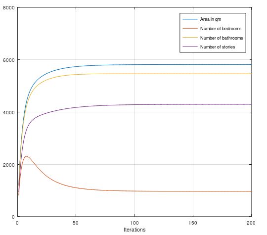
The benefit of the regularization term will be presented on the variable “parking lots” as an example. In the original dataset the impact on the price seems to be normal distributed. Meaning the more parking lots doesn’t increase the price for the house. Even with the default regression (regularization term deactivated) it is not clearly visible. But the assumption is that that the number of parking lots will increase the price. So with an respective λ-value this assumption can be introduced.
% Bayesian Regression activated
lambda_b = [0.0; 0.0; 0.0; 0.0; 0.0; 0.0; 0.0; 0.0; 0.0; 0.0; -0.002; 0.0; 0.0;];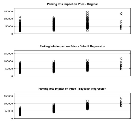
Finally after the regression model calculated example data can be used to obtain a price based on these data. Note that the previous scaled data need to be converted back to receive the correct price.
p = zeros(1,V);
p(1) = 300; %area: qm
p(2) = 2; %bedrooms
p(3) = 2; %bathrooms
p(4) = 2; %stories: number of levels
p(5) = 0; %main road: house faces main road
p(6) = 2; %guestroom: no: 0, yes: 1
p(7) = 1; %basement: no: 0, yes: 1
p(8) = 1; %hotwaterheating: house uses gas: no: 0, yes: 1
p(9) = 0; %airconditioning: no: 0, yes: 1
p(10) = 3; %parking: number of parking lots
p(11) = 0; %prefarea: house located in preferred area: no: 0, yes: 1
p(12) = 1; %furnishingstatus: furnished: 2, semi-furnished: 1, unfurnished: 0

p_s(1) = 1;
for i=2:V+1
   p_s(i) = (p(i-1) - mean(i-1)) / dev(i-1);
end

% Regression sample result
Y_p = p_s * h;The price for some sampled data is shown in the table below
| Area in qm | Bedrooms | Bathrooms | Stories | Main Road | Guestrooms | Basement | Gas Heating | Air Conditioning | Parking | Preferred Area | Furnishing | Price in Euro |
|---|---|---|---|---|---|---|---|---|---|---|---|---|
| 600 | 2 | 2 | 2 | 1 | 1 | 1 | 1 | 0 | 2 | 0 | 1 | 93256 |
| 1100 | 4 | 3 | 2 | 0 | 2 | 1 | 1 | 0 | 3 | 1 | 2 | 138930 |
| 300 | 1 | 1 | 0 | 1 | 0 | 1 | 1 | 0 | 1 | 0 | 0 | 44516 |
| 900 | 2 | 2 | 1 | 0 | 1 | 0 | 0 | 1 | 2 | 1 | 2 | 96544 |
The corresponding matlab code used in this example can be downloaded here.
Multiple linear regression is a powerful statistical method that helps in understanding and predicting the relationship between a dependent variable and multiple independent variables. By accurately estimating the regression coefficients, we can interpret the influence of each predictor and make informed decisions based on the model.
Polynomial (Nonlinear) Regression
Polynomial regression is a type of regression analysis in which the relationship between the independent variable X and the dependent variable Y is modeled as an k-th degree polynomial. This method extends linear regression by allowing for the possibility of a non-linear relationship between the variables, while still being linear in the parameters.
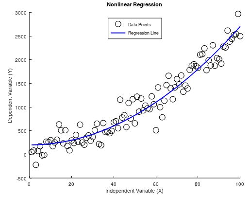
Polynomial regression includes polynomial terms x2, x3, …, xk-1 as predictors in addition to the linear term x. The general form of a polynomial regression model of degree is:
\hat{y} = \theta_0 + \theta_1 \: x + \theta_2 \: x^2 + ... +\theta_N \: x^N \:\: \rightarrow \:\: \hat{Y} = \Theta^T \: X\\[10pt]
\hat{Y}_{1,n} =\Theta^T_{1,k} \: X_{k,n} \:\: \xrightarrow{k=3} \:\: \hat{Y}_{1,n} =\begin{bmatrix}
\theta_0 & \theta_1 & \theta_2 \\
\end{bmatrix} \: \begin{bmatrix}
1 & 1 & \dots & 1 \\
x^{(1)} & x^{(2)} & \dots & x^{(n)} \\
x^{2(1)} & x^{2(2)} & \dots & x^{2(n)} \\
\end{bmatrix}\\[5pt]
Higher degree polynomials can fit more complex curves. However, increasing the degree too much can lead to overfitting, where the model fits the training data very well but performs poorly on new, unseen data.
Logistic Regression
Logistic regression is a statistical method used for binary classification, which means it predicts the probability that a given input belongs to one of two possible classes. Unlike linear regression, which predicts a continuous outcome, logistic regression predicts discrete outcomes (e.g., yes/no, true/false, spam/not spam). The model achieves this by modeling the relationship between the independent variables and the probability of the dependent variable using a logistic function (also known as the sigmoid function).
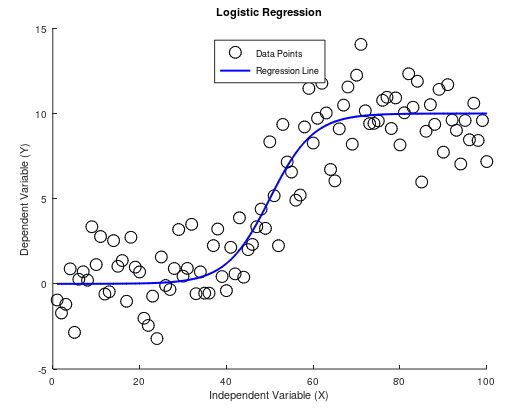
The logistic function transforms any real-valued number into a value between 0 and 1, which can be interpreted as a probability. The function is defined as:
\hat{y} = \frac{1}{1+e^{-(\theta_0 + \theta_1 x)}} = \frac{1}{1+e^{-\theta^T X}} \:\: \rightarrow \:\: \hat{Y} = h\left(\Theta^T \: X\right)\\[10pt]
\hat{Y}_{1,n} =h\left(\Theta^T_{1,k} \: X_{k,n}\right) \:\: \xrightarrow{k=2} \:\: \hat{Y}_{1,n} =h\left(\begin{bmatrix}
\theta_0 & \theta_1 \\
\end{bmatrix} \: \begin{bmatrix}
1 & 1 & \dots & 1 \\
x^{(1)} & x^{(2)} & \dots & x^{(n)} \\
\end{bmatrix}\right)\\[5pt]
The dependent variable y follows the binomial distribution where the probability of k successes in n independent Bernoulli trials where each trial have a probability of p will be calculated as followed:
B(k|p,n)=p(k)=\binom{n}{k}p^k(1-p)^{n-k}The binomial coefficient can be ignored to calculate the log based maximum location:
p(k)\sim p^k(1-p)^{n-k}\\[5pt]
ln\left(p^k(1-p)^{n-k}\right)=k \:\:ln(p)+(n-k)\:\:ln(1-p)\\[5pt]
In analogy to logistic regression the probability above represents the probability of y based on the probability of each sample (trial) prediction:
B(k=y|p=\hat{y},n=1)\rightarrow ln\left(p(y|h(\Theta^T \: X),1)\right)=y \:\:ln\left(h(\Theta^T \: X)\right)+(1-y)\:\:ln\left(1-h(\Theta^T \: X)\right)As discussed in the Multiple Linear Regression chapter above the cost function for the Logistic Regression is based on log-likelihood as shown below:
J(\Theta)=-\frac{1}{N}\sum_{n=1}^{N}\left(y^{(n)}\:\:ln\left(h_\Theta(x^{(n)}\right)+(1-y^{(n)})\:\:ln\left(1-h_\Theta(x^{(n)}\right)\right)A numerical solution (not part of this blog) helps to calculate the max-likelihood equation and finally it comes out that this equation is the same as for calculated for the Multiple Linear Regression.
\frac{\partial J(\Theta)}{\partial\Theta}=\frac{1}{N}\sum_{n=1}^{N}\left(h_\Theta(x^{(n)})-y^{(n)}\right)x^{(n)}\\[5pt]For the max-likelihood calculation see the Gradient Descent Algorithm discussed above based on same max-likelihood equation as used in Multiple Linear Regression.
Example
To demonstrate the Logistic Regression the dataset Heart Disease Prediction from https://www.kaggle.com/ homepage will be used.
An extraction of the data content some rows are shown in the table below.
| Male | Age | Education | Current Smoker | Cigarettes per Day | Blood Pressure Medication | Prevalent Stroke | Prevalent Hypertensive | Diabetes | Total Cholesterol | Systolic Blood Pressure | Diastolic Blood Pressure | BMI | Heart Rate | Glucose Level | Risk of Heart Disease |
|---|---|---|---|---|---|---|---|---|---|---|---|---|---|---|---|
| 1 | 43 | 1 | 1 | 30 | 0 | 0 | 1 | 0 | 225 | 162 | 107 | 23.61 | 93 | 88 | 0 |
| 0 | 46 | 2 | 1 | 20 | 0 | 0 | 0 | 0 | 291 | 112 | 78 | 23.38 | 80 | 89 | 1 |
| 1 | 57 | 1 | 0 | 0 | 0 | 0 | 0 | 0 | 220 | 136 | 84 | 26.84 | 75 | 64 | 1 |
| 1 | 41 | 4 | 1 | 43 | 0 | 0 | 0 | 0 | 252 | 124 | 86 | 28.56 | 100 | 70 | 0 |
| 0 | 60 | 1 | 0 | 0 | 0 | 0 | 1 | 1 | 258 | 142 | 87 | 32.53 | 82 | 145 | 0 |
| : | : | : | : | : | : | : | : | : | : | : | : | : |
A more detailed description of the table columns is available in following matlab code.
Note that it is very important before starting with the regression calculations that all data are scaled according to the Gaussian (normal) distribution mean value to be zero and standard deviation to be one. Otherwise the data are not comparable and the regression will fail.
R = dlmread("framingham_heart_disease.csv",";");
L = 3656;
V = 15;
x = zeros(15,L);
x(1,:) = R(:,1)'; %male: 1, female: 0
x(2,:) = R(:,2)'; %age
x(3,:) = R(:,3)'; %education: 1…no graduation, 2...secondary school certificate,
                            % 3…secondary school diploma, 4…high school
x(4,:) = R(:,4)'; %current smoker
x(5,:) = R(:,5)'; %cigarettes per day
x(6,:) = R(:,6)'; %blood presure medication
x(7,:) = R(:,7)'; %prevalent stroke
x(8,:) = R(:,8)'; %prevalent hypertensive
x(9,:) = R(:,9)'; %diabetes
x(10,:) = R(:,10)'; %total cholesterol: >240…Dangerous, 200…239 At risk, <200 Heart healthy
x(11,:) = R(:,11)'; %systolic blood pressure
x(12,:) = R(:,12)'; %diastolic blood pressure
x(13,:) = R(:,13)'; %BMI
x(14,:) = R(:,14)'; %heart rate
x(15,:) = R(:,15)'; %glucose level: >110 pathological, 60…109 normal
y = R(:,16)'; %ten years risk of heart disease

mean = zeros(1,V);
mean_s = zeros(1,V);
x_s = zeros(V+1,L);

%Scaling needed for every feature vector
%Mean value = 0, standard deviation = 1
for i=1:V
   mean(i) = sum(x(i,:)/L);
   dev(i) = sqrt(sum((x(i,:)-mean(i)).^2)/L);
   x_s(i+1,:) = (x(i,:) - mean(i)) / dev(i);
   mean_s(i) = sum(x_s(i+1,:)/L);
   dev_s(i) = sqrt(sum((x_s(i+1,:)-mean_s(i)).^2)/L);
endThe gradient descent algorithm is shown in following matlab code. Using a step width of beta = 0.0002 about 300 iterations are sufficient to have the parameter settled.
The Bayesian based regularization term is deactivated actually.
it = 300;
beta = 0.0002;

x_s(1,:) = 1;
X = x_s';

% Bayesian Regression deactivated
lambda = [0.0; 0.0; 0.0; 0.0; 0.0; 0.0; 0.0; 0.0; 0.0; 0.0; 0.0; 0.0; 0.0; 0.0; 0.0; 0.0;];

h_trend = zeros(V+1,it);
for i=1:it
  H = 1 ./ (1 + exp(-(X * h)));
  h = h - beta * ((X' * H) - (X' * y') + (lambda * h' * h ));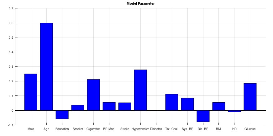
endThe result of the model parameter h is shown below. These parameters represent the factor of each category how strong or weak is the impact on the 10 years risk of heart disease. In this blog it is not intended to give any medicine recommendation but it seems that the age, male, cigarettes, blood pressure and glucose level has biggest impact on the risk.
Finally after the parameter model calculated example data can be used to predict the 10 years risk of heart disease on these data. Note that the previous scaled data need to be converted back to receive the correct result.
p = zeros(1,V);
p(1) = 0; %male: 1, female: 0
p(2) = 65; %age
p(3) = 4; %education: 1…no graduation, 2...secondary school certificate,
                            % 3…secondary school diploma, 4…high school
p(4) = 1; %current smoker
p(5) = 10; %cigarettes per day
p(6) = 1; %blood presure medication
p(7) = 1; %prevalent stroke
p(8) = 1; %prevalent hypertensive
p(9) = 1; %diabetes
p(10) = 200; %total cholesterol: >240…Dangerous, 200…239 At risk, <200 Heart healthy
p(11) = 170; %systolic blood pressure
p(12) = 110; %diastolic blood pressure
p(13) = 70; %BMI
p(14) = 90; %heart rate
p(15) = 150; %glucose level: >110 pathological, 60…109 normal

p_s(1) = 1;
for i=2:V+1
   p_s(i) = (p(i-1) - mean(i-1)) / dev(i-1);
end

% Regression sample result
Y_p = 1 ./ (1 + exp(-(p_s * h)));The 10 years risk for some sampled data is shown in the table below. Note that the risk of 1 means 100% risk.
| Male | Age | Education | Current Smoker | Cigarettes per Day | Blood Pressure Medication | Prevalent Stroke | Prevalent Hypertensive | Diabetes | Total Cholesterol | Systolic Blood Pressure | Diastolic Blood Pressure | BMI | Heart Rate | Glucose Level | Risk of Heart Disease |
|---|---|---|---|---|---|---|---|---|---|---|---|---|---|---|---|
| 1 | 75 | 1 | 1 | 40 | 1 | 1 | 1 | 0 | 260 | 165 | 90 | 33.0 | 80 | 110 | 0.869 |
| 0 | 50 | 3 | 0 | 0 | 0 | 0 | 0 | 0 | 150 | 115 | 80 | 22.0 | 80 | 90 | 0.054 |
| 1 | 55 | 2 | 1 | 15 | 1 | 0 | 1 | 1 | 220 | 140 | 85 | 26.0 | 75 | 80 | 0.372 |
| : | : | : | : | : | : | : | : | : | : | : | : | : |
The corresponding matlab code used in this example can be downloaded here.

Hey people!!!!!
Good mood and good luck to everyone!!!!!
Hey people!!!!!
Good mood and good luck to everyone!!!!!