Adaptive Filter

At its core, an adaptive filter is a digital filter that adjusts its parameters based on the input it receives. Unlike traditional fixed filters with static coefficients, adaptive filters dynamically alter their settings to optimize performance in changing environments. This adaptability is what sets them apart, allowing them to excel in scenarios where the characteristics of the input signal may vary over time.
The magic of adaptive filters lies in their ability to learn and adapt. The two primary components driving this capability are the filter coefficients and the adaptation algorithm. The filter coefficients represent the adjustable parameters that the filter tunes to optimize its response, while the adaptation algorithm governs the adjustment process.
The working principle involves a continuous feedback loop: the adaptive filter processes the input signal, compares the output with the desired signal, computes the error, and adjusts its coefficients accordingly. This iterative process continues until the filter converges to an optimal configuration.

Filter structure

The structure of an adaptive filter is composed of key components that work together to dynamically adjust and optimize the filter’s behavior based on input signals. Here’s a breakdown of the typical structure of an adaptive filter:

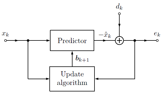
The adaptive filter begins its process by receiving an input signal, denoted as x_k. This signal is the raw data or the signal that requires processing or enhancement. It could be a noisy audio signal, a distorted communication signal, or any other type of signal that needs refinement.
At the heart of the adaptive filter are the filter coefficients, represented by the vector b_k. These coefficients determine how the input signal is filtered. Unlike traditional filters with fixed coefficients, adaptive filters have the ability to adjust these coefficients iteratively based on the input and desired output.
The result of the Predictor is the output signal which represents the filtered version of the input. In the initial stages, when the filter is not yet optimized, this output may not match the desired signal accurately.
The desired signal, d_k, serves as a reference for the adaptive filter. It represents the ideal or target output that the filter aims to achieve. The difference between the actual output and the desired output is used to compute the error e_k.
The Update algorithm is the intelligence behind the adaptive filter. It governs how the filter coefficients are adjusted in response to the error signal. Common algorithms include the Least Mean Squares (LMS) algorithm and Recursive Least Squares (RLS) algorithm. These algorithms use the error signal to update the filter coefficients, gradually minimizing the error over time.

Predictor

To estimate the desired signal d_k based on the history of the input signal x_k a so called Predictor is used. The Predictor is commonly implemented as a FIR (Finit Input Response) Filter. Its structure for a 3rd order Filter is shown below:

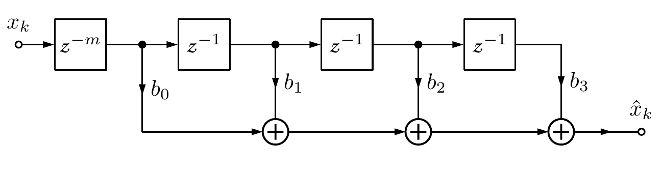
With the Z-Transformation a difference equation as a sum operation will be obtained.

H(z)=\frac{\hat{X}(z)}{X(z)}=\sum_{i=0}^{N} b_i\:z^{-i-m}=b_0z^{-m}+b_1z^{-1-m}+\dots+b_Nz^{-N-m}\:\:
\origof \:\:\hat{x}_k=\sum_{i=0}^{N} b_i\:x_{k-i-m}\\[5pt]

The z^-m block is used to delay the input values so that the signal can be preticted based on past values. An ideal Predictor estimates the desired signal d_k in the way that the resulting error e_k is equal to zero.

e_k=d_k-\hat{x}_k\\[5pt]

Update Algorithm

To find the coefficients b_k the Least Mean Squares Algorithm (LMS) is a common method. This algorithm is a widely used adaptive filtering algorithm that aims to minimize the mean squared error between the desired signal and the output of the adaptive filter. It’s a stochastic gradient descent algorithm that iteratively adjusts the filter coefficients based on the instantaneous error.

The gradient descent method is described as followed:

\textit{\textbf{b}}_{k+1}=\textit{\textbf{b}}_k-\beta \frac{\partial E(e_k^2)}{\partial \textit{\textbf{b}}_k}\\[10pt]

Calculation of the step size β

The step size β defines the steps towards the optimium of the coefficients. The bigger the value the faster the optimun can be found. On the other hand the probability is increased to jump over the optimum.

E(e_k^2) = \frac{1}{N}\sum_{k=0}^{N-1}\left(x_k-\textit{\textbf{b}}_k\textit{\textbf{X}}_k\right)^2=E\left(\left(x_k-\textit{\textbf{b}}_k\textit{\textbf{X}}_k\right)^2\right)\\[10pt]
E(e_k^2) = E(x_k^2)-2\textit{\textbf{b}}_k E(\textit{\textbf{X}}_k)+\textit{\textbf{b}}_k^T E(\textit{\textbf{X}}_k^2)\textit{\textbf{b}}_k\\[10pt]
\frac{\partial E(e_k^2) }{\partial \textit{\textbf{b}}_k}= -2 \underbrace{E(\textit{\textbf{X}}_k)}_\text{\clap{mean value free}}+2 \textit{\textbf{b}}_k \underbrace{E(\textit{\textbf{X}}_k^2)}_\text{\clap{$R_{xx,k}$}}=2\textit{\textbf{R}}_{xx,k}\textit{\textbf{b}}_k\\[10pt]
\frac{\partial E(e_k^2)}{\partial \textit{\textbf{b}}_k} \approx \frac{\Delta E(e_k^2)}{\Delta \textit{\textbf{b}}_k}=2\textit{\textbf{R}}_{xx,k}\left(\textit{\textbf{b}}_k-\textit{\textbf{b}}_{k-1}\right)\\[10pt]

Inserted into the gradient descent equation from above the result is as followed:

\textit{\textbf{b}}_{k+1}=\textit{\textbf{b}}_k-2\beta \textit{\textbf{R}}_{xx,k}\left(\textit{\textbf{b}}_k-\textit{\textbf{b}}_{k-1}\right)

Looking into a system with 2 coefficients (2nd order filter) the gradient of the coefficients will go to zero in case of an optimum.

\textit{\textbf{b}}_{k+1} = \textit{\textbf{b}}_{k-1}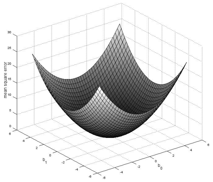

So the equation from above can be simplified.

\beta=\frac{1}{2}\:I\:\textit{\textbf{R}}_{xx,k}^{-1} \xrightarrow{n\:x\:n} \beta=\frac{1}{2}\:\textit{\textbf{R}}_{xx,k}^{-1}

So step size β should be in following range:

0 < \beta < \textit{\textbf{R}}_{xx,k}^{-1}

A Convergence will happen for the sum of the intrinsic values of Correlation Matrix R_xx,k.

(N+1)\:R_{xx}(0)=(N+1)\:\sigma_{xx}^2 \rightarrow 0 < \beta < \frac{1}{(N+1)\:\sigma_{xx}^2}

Calculation of the descent gradient

The descent gradient is defined by the partial differentation of error signal expectation against the filter coefficients. The descent gradiant can be calculated with the help of following mathmatical transformations shown below:

\frac{\partial E(e_k^2)}{\partial \textit{\textbf{b}}_k}=E\left(\frac{\partial e_k^2}{\partial \textit{\textbf{b}}_k}\right)\\[10pt]
\frac{\partial e_k^2}{\partial \textit{\textbf{b}}_k}=2e_k\frac{de_k}{d \textit{\textbf{b}}_k}\\[10pt]
e_k=x_k-\textit{\textbf{b}}_k \textit{\textbf{X}}_k\\[10pt]
\frac{\partial e_k^2}{\partial \textit{\textbf{b}}_k}=2e_k(-\textit{\textbf{X}}_k)\\[10pt]
\frac{\partial E(e_k^2)}{\partial \textit{\textbf{b}}_k}=-2E(e_k\textit{\textbf{X}}_k)=-2e_k \frac{1}{N}\sum_{i=0}^{N-1}\textit{\textbf{X}}_{k-i}\xrightarrow{N=1}-2e_k\textit{\textbf{X}}_k\\[10pt]

Finally the update algorithm can be summarized as followed:

\textit{\textbf{b}}_{k+1}=\textit{\textbf{b}}_k+\beta\:2e_k\textit{\textbf{X}}_k\\[10pt]
0 < \beta < \frac{1}{(N+1)\:\sigma_{xx}^2}

Echo and Noise Cancellation

The performance of the adaptive filter will be shown based on a Loudspeaker to suppress the echo and noise coupled back into Microphone.

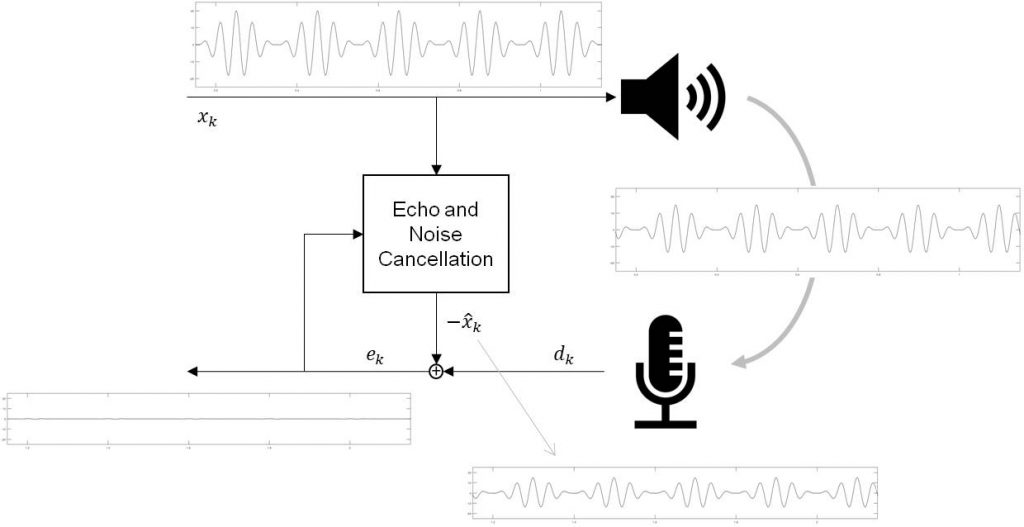
Behind the block “Echo and Noise Cancellation” there is the adaptive filter located discussed in previous chapter above. Lets assume a “Noise” signal on x_k consisting of two sinus signals causing the frequency response (blue line) below. This signal is coupled in to the Micro with some delay (echo). The task of the filter is to eliminate this Noise signal on e_k. Error e_k signal might be not the right wording since it is not about an Error signal but a Microphone signal. Just to keep the same term not to cause any confusion.

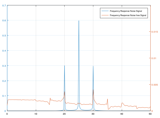
The filters result is shown on e_k signal and on frequency response red line above. Note that the filters delay z^-m has to be used to adapt the filter on the Echo happened by the signal coupling into the Microphone. Finally a damping of the Noise signal of about -43dB can be achieved.
Below the Matlab code of the algorithm including the Noise signal generation is shown. The corresponding m-file can also be downloaded here.

% The sampling frequency in Hz.
Fs = 1000;
% Sampling time
T = 1/Fs;
% Buffer length
M = 4000;
% Create a time base
t = (0:M-1)*T;
% Loudspeaker signal
x = (5*sin((5*6.28*t))+5).*(2*sin(25*6.28*t));
% Loudspeaker signal coupled into Microphone (delayed and damped)
x_echo = (5*sin(5*(6.28*t-0.3))+5).*(1.5*sin(25*(6.28*t-0.3)));
% Desired signal
d = x_echo;
% Predictor order (FIR filter order + 1)
p = 32
% Initialize Coefficients
b = zeros(p,1);
N  = length(b)-1;
% Signal length
Lx = length(x);
% Init length
x_init = x(1:500);
Lx_init = length(x_init);
% Initial cross correlation of Loudspeaker signal
Rx = xcorr(x_init,'unbiased');
rx0 = Rx(Lx_init);
disp(Rx(Lx_init));
% Initialize output and error
y = zeros(1,Lx);
e = zeros(1,Lx+1);
% Compensation delay
delay = 230;

for k = 1:Lx
    % Update coefficients after Initialization
    if k > (Lx_init+delay)
      % Update correlation value
      rx1 = rx0 + ((1/Lx_init)*((x(k-delay)*x(k-delay))-rx0));
      % Calculate Step size with a factor of 0.2
      beta = 1/(rx1*(p+1)*5);
      % Take input values based on number of coefficients
      xn  = x(k-delay:-1:k-N-delay)';
      % Update filter coefficients
      b = b + 2*beta*e(k)*xn;
      % Predict the desired signal
      y(k) = x(k-delay:-1:k-N-delay)*b;
      % Calculate the difference between desired and predicted signal
      e(1+k) = d(k) - y(k);
      % Buffer old correlation value
      rx0 = rx1;
    endif
end